Audio gallery
Listenable examples across three cetacean species, drawn live from the remote
data catalog that ships with the toolkit. These are the clips decipher.fetch(...) returns — use them to calibrate your ear
before pointing the primitives at your own recordings.
from decipher import fetch,
written back out with write_wav, and rendered with render_spectrogram — one toolkit round-trip per asset.Humpback whale — Megaptera novaeangliae
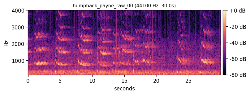
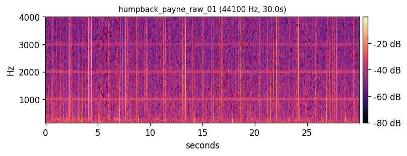
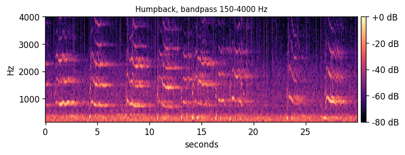
Long, tonal song phrases. Most energy sits in 200-2000 Hz; structure is hierarchical (units → phrases → themes). Source: Payne & McVay 1971 corpus, 44.1 kHz.
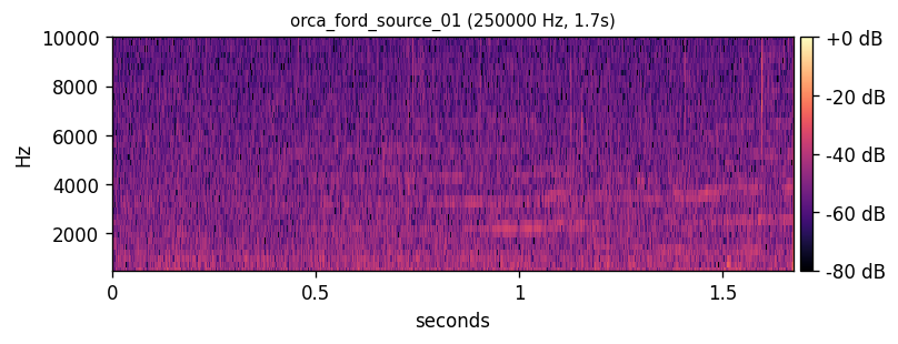
Killer whale (orca) — Orcinus orca
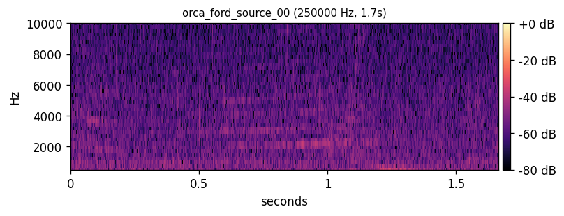
Short, stereotyped pulsed calls organized into population-specific dialects. Most call energy is in 500-5000 Hz but the recordings are sampled at 250 kHz to also capture echolocation clicks. Source: Ford 1991 / LimeKiln hydrophone.
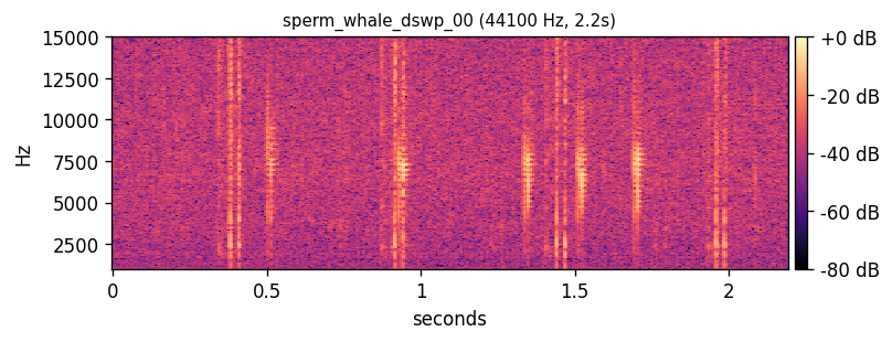
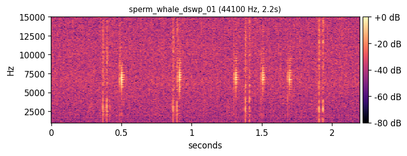
Sperm whale — Physeter macrocephalus
Codas: short rhythmic patterns of broadband clicks. Each coda is characterised by inter-click intervals and total duration rather than spectral content. Source: Sharma 2024 / Dominica Sperm Whale Project HF.
Segmented units
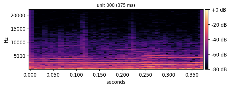
Running detect_units on the first humpback excerpt produced
18 energy-bounded units. Each is a listenable Unit object
with start_s, end_s, and its own source_samples — the round-trip invariant in miniature.
Reproducing this page
from decipher import fetch, bandpass, detect_units, write_wav
from decipher.audio import render_spectrogram

# Three species, two clips each
humpback = fetch(paper_id="001_payne_mcvay_1971",
                 substrate="humpback_song_raw", limit=2)
orca     = fetch(paper_id="004_ford_1991",
                 substrate="ford_source_clips", limit=2)
sperm    = fetch(paper_id="005_sharma_2024",
                 substrate="DSWP-HF",
                 min_duration_s=0.5, max_duration_s=5.0, limit=2)

# Round-trip: bandpass the first humpback and save it
bp = bandpass(humpback[0].samples, humpback[0].sr, 150.0, 4000.0)
write_wav("humpback_bandpassed.wav", bp, humpback[0].sr)

# Segment into listenable units
units = detect_units(humpback[0].samples, humpback[0].sr)
for u in units[:5]:
    write_wav(f"unit_{u.index:03d}.wav", u.source_samples, u.sr)