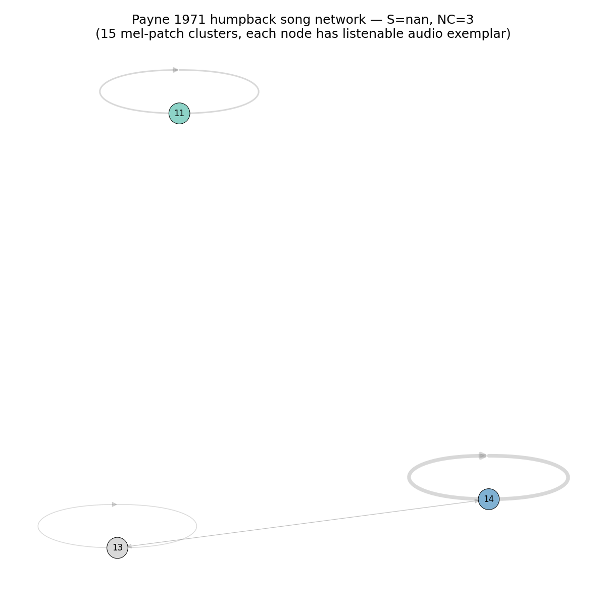
Tutorial 6 — Zipf and Menzerath

Two predictions from linguistic-efficiency theory, applied to your symbol stream.

Zipf's law of abbreviation

Prediction: more frequent element types tend to be shorter. Implemented as a mixed-effects model with (1 | type) random intercepts:

from decipher import zipf_brevity_test

# durations[i] is the duration in seconds of element i;
# types[i] is the type label (e.g. cluster id) of element i.
durations = [u.duration_s for u in units]
types     = [int(s) for s in stream.symbols]

result = zipf_brevity_test(durations=durations, types=types)
print(result.count_estimate, result.ci_lo, result.ci_hi, result.holds)

holds is True iff the entire 95% Wald CI is below zero — strong evidence for the law.

Menzerath's law

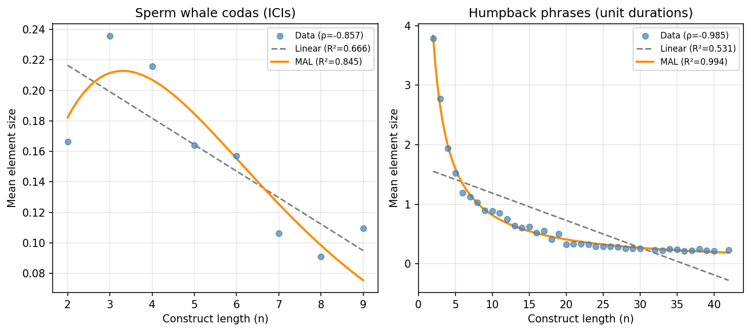
Prediction: longer sequences consist of shorter elements. Implemented as scale(log(duration)) ~ scale(log(length)) + (1|sequence).

from decipher import menzerath_test

# sequences is a list of lists of (duration_s) per element;
# each inner list is one sequence (e.g. one song theme).
sequences = [...]   # list[list[float]]

result = menzerath_test(sequences)
print(result.length_estimate, result.ci_lo, result.ci_hi, result.holds)
print("position effect:", result.position_estimate, result.position_ci_lo, result.position_ci_hi)

Zipf rank-frequency fit

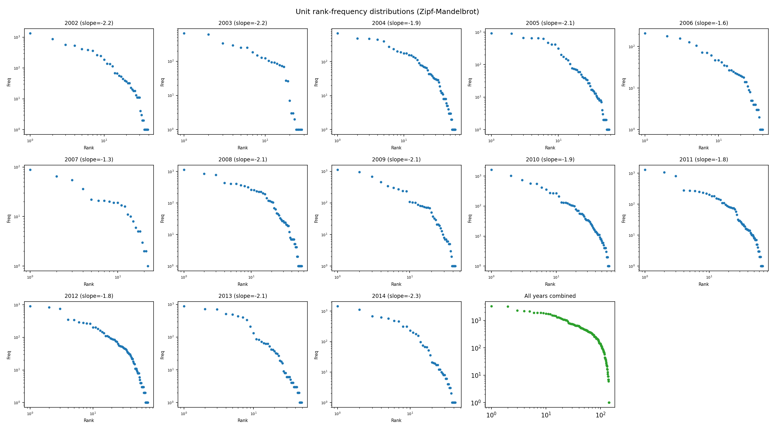
For the rank-frequency power law itself (independent of duration):

from decipher import zipf_frequency_fit

counts = [...]    # type counts, e.g. from collections.Counter on stream.symbols
fit = zipf_frequency_fit(counts)
print(fit)

n-gram perplexity and bigram transitions

from decipher import ngram_perplexity, bigram_transitions

ng = ngram_perplexity(sequences=[list(map(str, stream.symbols))], n=3, smoothing_k=0.1)
print(ng.perplexity, ng.entropy_bits)

tc = bigram_transitions(sequences=[list(map(str, stream.symbols))])
matrix, vocab = tc.as_matrix()
print(tc.probability("3", "5"))