Guide — Spectrograms

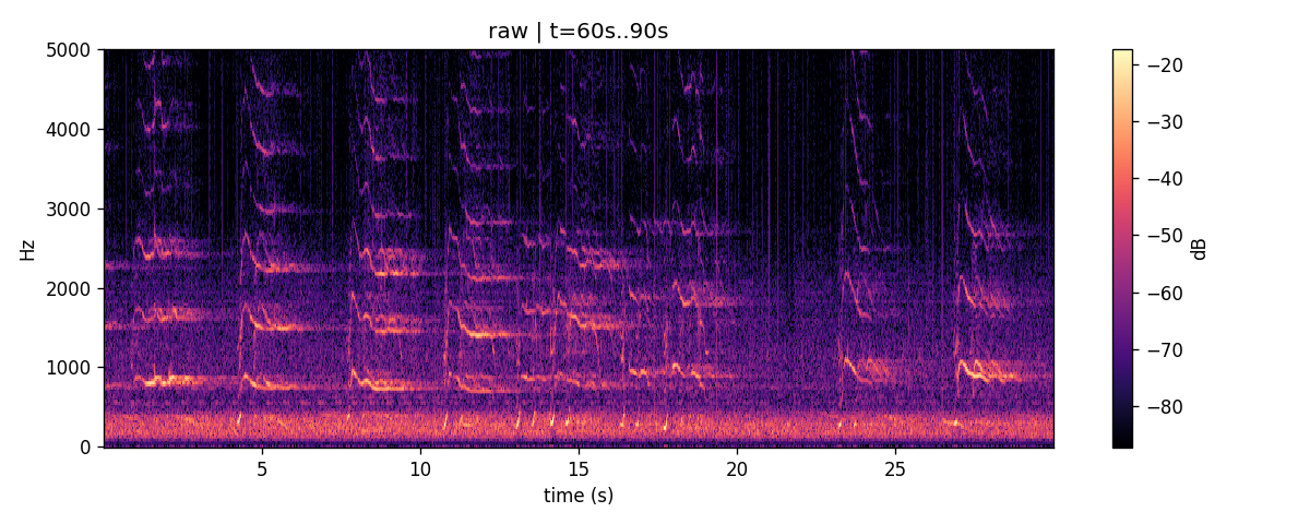
Render an STFT spectrogram for any clip with a single call.

render_spectrogram

from decipher.audio import render_spectrogram

render_spectrogram(
    audio=src.samples, sr=src.sr,
    out_path="figures/excerpt_00.png",
    lo_hz=20, hi_hz=4000,
    n_fft=1024, hop=256,
    title="excerpt 00",
    width_px=800, height_px=300, dpi=120,
)

The function is a thin wrapper over librosa's STFT and matplotlib. The lo_hz / hi_hz parameters bound the y-axis only — the FFT itself is full-bandwidth.

Why it lives in the toolkit

Every paper reproduction needs per-clip spectrograms with the same recipe (STFT → log magnitude → imshow with a frequency axis). Standardising the rendering keeps figures visually consistent across papers and lets the documentation, the planner, and the per-paper figure scripts call the same function.

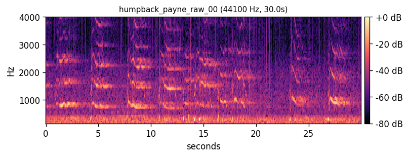
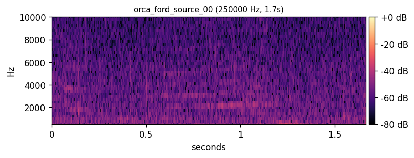
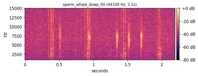
Three species, three acoustic regimes

Same call (render_spectrogram), very different pictures. Click play to hear what the y-axis is actually showing.

44.1 kHz source; rendered with lo_hz=20, hi_hz=4000. 44100 Hz

250 kHz source; display capped at 10 kHz to show the audible band. 250000 Hz

44.1 kHz source; the spectrogram looks like vertical stripes because each click is near-instantaneous. 44100 Hz

Choosing FFT parameters

For most cetacean work the defaults are fine. For infrasonic blue-whale calls or very narrow-band clicks, use auto_mel_params first to get species-appropriate FFT parameters, then pass the same n_fft / hop to render_spectrogram so the figure matches the features.